An application of convolution in machine learning#
Convolution and cross-correlation operations play a crucial role in computer vision and machine learning, particularly in tasks like visual recognition. Let us delve into a practical application of convolution in hand-written digit recognition.
For this, we will use the MNIST dataset. Here are important details about this dataset:
10 classes,
60 thousand training images,
10 thousand testing images,
Each image is monochrome, 28-by-28 pixels.
Sample MNIST images:

We will use the PyTorch library, which will take care of the optimization, auto-differentiation, etc.
#@title Import the required modules
import torch
import torch.nn as nn
import torchvision.datasets as datasets
import torchvision.transforms as transforms
# Define the "device". If GPU is available, device is set to use it, otherwise CPU will be used.
device = torch.device('cuda:0' if torch.cuda.is_available() else 'cpu')
The following code will download the MNIST dataset.
#@title Download the dataset
train_data = datasets.MNIST(root = './data', train = True,
                        transform = transforms.ToTensor(), download = True)

test_data = datasets.MNIST(root = './data', train = False,
                       transform = transforms.ToTensor())
As we describe in Section 4.3 of the book, here we are only interested in binary classification, that is, we deal with only two classes. We pick “3” as the positive (target) class and all remanining digits as the negative class.
target_class = 3

train_data.targets[train_data.targets!=target_class] = 0
train_data.targets[train_data.targets==target_class] = 1

test_data.targets[test_data.targets!=target_class] = 0
test_data.targets[test_data.targets==target_class] = 1
# About the ToTensor() transformation.

# PyTorch networks expect a tensor as input with dimensions N*C*H*W  where
# N: batch size
# C: channel size
# H: height
# W: width

# Normally an image is of size H*W*C.
# ToTensor() transformation moves the channel dimension to the beginning as needed by PyTorch.
Let us define the data loaders. This takes care of shuffling and splitting the dataset into mini-batches.
#@title Define the data loaders
batch_size = 100
train_loader = torch.utils.data.DataLoader(dataset = train_data,
                                             batch_size = batch_size,
                                             shuffle = True)

test_loader = torch.utils.data.DataLoader(dataset =  test_data ,
                                      batch_size = batch_size,
                                      shuffle = False)
The following piece of code defines our neural network. It consists of a single “conv” layer, which essentially implements the cross-correlation operation. Its kernel (filter) size is 28x28, so, its weigths fully covers the input image. We are interested in computing:
where x is the input image and h represent the weights of the “conv” layer. The output of this layer is then passed through a sigmoid layer:
#@title Define a CNN network

class CNN(nn.Module):
    #This defines the structure of the NN.
    def __init__(self):
        super(CNN, self).__init__()
        self.conv1 = nn.Conv2d(1, 1, kernel_size=28, bias=False)
        self.sig = nn.Sigmoid()

    def forward(self, x):
        x = self.conv1(x)
        x = self.sig(x.view(-1, 1))
        return x


# Create an instance
net = CNN().to(device)

print(net)
CNN(
  (conv1): Conv2d(1, 1, kernel_size=(28, 28), stride=(1, 1), bias=False)
  (sig): Sigmoid()
)
Next, we define the loss function and the optimization method.
#@title Define the loss function and the optimizer
loss_fun = nn.MSELoss()
optimizer = torch.optim.SGD( net.parameters(), lr=0.001, momentum=.9)
The following piece of code trains the network (i.e. the “conv” layer). There are two loops; the first of which passes through the whole dataset, the second passes through the mini-batches. For each mini-batch, we run the model using its current weights, compute loss, compute the gradient vector of the weights of the conv layer and then update them.
#@title Train the model
losses = []
iter_nums = []
num_epochs = 7
for epoch in range(num_epochs):
  for i ,(images,labels) in enumerate(train_loader):
    images = images.to(device)
    labels = labels.to(device)
    labels = labels[:,None].float()

    optimizer.zero_grad()
    output = net(images) # runs the model
    loss = loss_fun(output, labels)  # computes loss
    loss.backward()  # computes the gradient of the weights
    optimizer.step()  # update weights (backpropagation)

    # if epoch==4:
    #   optimizer = torch.optim.SGD( net.parameters(), lr=0.0001, momentum=.9)

    if (i+1) % batch_size == 0:
      losses.append(loss.item())
      iter_nums.append(epoch*len(train_loader)+i)
      print('Epoch [%d/%d], Step [%d/%d], Loss: %.4f'
                 %(epoch+1, num_epochs, i+1, len(train_data)//batch_size, loss.item()))
Epoch [1/7], Step [100/600], Loss: 0.0727
Epoch [1/7], Step [200/600], Loss: 0.0700
Epoch [1/7], Step [300/600], Loss: 0.0850
Epoch [1/7], Step [400/600], Loss: 0.0757
Epoch [1/7], Step [500/600], Loss: 0.1031
Epoch [1/7], Step [600/600], Loss: 0.0492
Epoch [2/7], Step [100/600], Loss: 0.0510
Epoch [2/7], Step [200/600], Loss: 0.0655
Epoch [2/7], Step [300/600], Loss: 0.0933
Epoch [2/7], Step [400/600], Loss: 0.0290
Epoch [2/7], Step [500/600], Loss: 0.0557
Epoch [2/7], Step [600/600], Loss: 0.0524
Epoch [3/7], Step [100/600], Loss: 0.0346
Epoch [3/7], Step [200/600], Loss: 0.0426
Epoch [3/7], Step [300/600], Loss: 0.0494
Epoch [3/7], Step [400/600], Loss: 0.0505
Epoch [3/7], Step [500/600], Loss: 0.0271
Epoch [3/7], Step [600/600], Loss: 0.0393
Epoch [4/7], Step [100/600], Loss: 0.0351
Epoch [4/7], Step [200/600], Loss: 0.0445
Epoch [4/7], Step [300/600], Loss: 0.0303
Epoch [4/7], Step [400/600], Loss: 0.0431
Epoch [4/7], Step [500/600], Loss: 0.0577
Epoch [4/7], Step [600/600], Loss: 0.0250
Epoch [5/7], Step [100/600], Loss: 0.0237
Epoch [5/7], Step [200/600], Loss: 0.0510
Epoch [5/7], Step [300/600], Loss: 0.0425
Epoch [5/7], Step [400/600], Loss: 0.0476
Epoch [5/7], Step [500/600], Loss: 0.0139
Epoch [5/7], Step [600/600], Loss: 0.0388
Epoch [6/7], Step [100/600], Loss: 0.0369
Epoch [6/7], Step [200/600], Loss: 0.0157
Epoch [6/7], Step [300/600], Loss: 0.0460
Epoch [6/7], Step [400/600], Loss: 0.0416
Epoch [6/7], Step [500/600], Loss: 0.0324
Epoch [6/7], Step [600/600], Loss: 0.0372
Epoch [7/7], Step [100/600], Loss: 0.0260
Epoch [7/7], Step [200/600], Loss: 0.0422
Epoch [7/7], Step [300/600], Loss: 0.0245
Epoch [7/7], Step [400/600], Loss: 0.0423
Epoch [7/7], Step [500/600], Loss: 0.0677
Epoch [7/7], Step [600/600], Loss: 0.0422
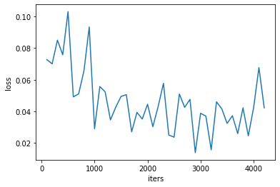
The following plots the loss over iterations.
import matplotlib.pyplot as plt

plt.plot(iter_nums,losses)
plt.xlabel('iters')
plt.ylabel('loss')
plt.show()
To evaluate the trained model, we run it on the test set and report percent accuracy.
#@title Run the trained model on the testing set

correct = 0
total = 0
for images,labels in test_loader:
  images = images.to(device)
  labels = labels.to(device)

  out = net(images)
  _, predicted_labels = torch.max(out,1)
  correct += (predicted_labels == labels).sum()
  total += labels.size(0)

print('Percent correct: %.3f %%' %((100*correct)/(total+1)))
Percent correct: 89.891 %
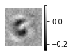
Let us now plot the learned weights. This should look like the positive class (whcih is “3” in our example).
from matplotlib import pyplot as plt
weights = net.conv1.weight.data.clone().cpu().numpy()
filter = weights.reshape(28,28)
plt.figure(i, figsize=(1.2,1.2))
plt.axis('off')
plt.imshow(filter, cmap='gray')
plt.colorbar()
<matplotlib.colorbar.Colorbar at 0x148dbcb80>
For the multiclass version of this exercise: click here.
Related content: