Convolution of two complex exponentials

Convolution of two complex exponentials#

Suppose that a CT LTI system is represented by the impulse response \(h(t)=e^{\lambda_2t}u(t)\). What would be the output of this system for input \(x(t)=e^{\lambda_1t}u(t)\)? The answer to this question is the convolution of \(h(t)\) and \(x(t)\):

\[ y(t) = x(t) * h(t)= \int_{-\infty}^\infty x(\tau) h(t-\tau) d\tau. \]

\(y(t) = \int_{-\infty}^\infty e^{\lambda_1 \tau}u(\tau) e^{\lambda_2 (t-\tau)}u(t-\tau) d\tau = \frac{e^{\lambda_1t}-e^{\lambda_2t}}{\lambda_1-\lambda_2}u(t).\) Refer to Exercise 4.5 in the book for the intermediate steps.

Let us verify this result for \(\lambda_1=-2\) and \(\lambda_2=-5\) using Sympy.

import sympy as sym

t, tau = sym.symbols('t tau', real=True)

# input signal 
x = sym.Piecewise((0, t<0),(sym.exp(-2*t), True)) 

# impulse response
h = sym.Piecewise((0, t<0),(sym.exp(-5*t), True))

# convolution
xtau = x.subs(t, tau)
htau = h.subs(t,tau)
y = sym.integrate(xtau*htau.subs(tau, t-tau), (tau, -sym.oo, sym.oo))
y

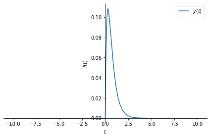
\[\displaystyle \frac{e^{- 2 t}}{3} - \frac{e^{- 5 t} e^{3 \min\left(0, t\right)}}{3}\]

The expression above is equivalent to \(\frac{e^{-2t}-e^{-5t}}{-2+5} u(t)\). The plot of \(y(t)\) is shown below.

sym.plot(y, label=r'$y(t)$',legend=True);

_images/f0ccca11751354e4f1bef625301003578d4f4f71792c0f1ae88e5064d2ff8b88.png

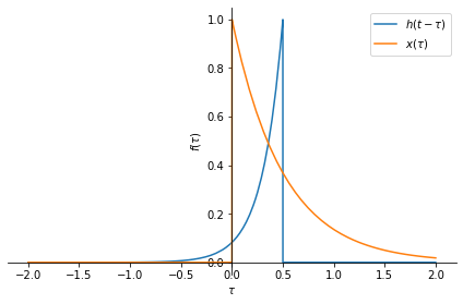
You can visualize and compute the values of this convolution integral at specific \(t\) values using the following code. \(y(t)\) is the area under \(h(t-\tau)\) weighted by \(x(\tau)\). You can try different \(t\) values below.

import numpy as np
t=.5
print("For t =",t)
p1 = sym.plot(xtau, (tau, -2, 2), show=False, label=r'$x(\tau)$', legend=True)
p2 = sym.plot(htau.subs(tau,t-tau), (tau, -2, 2), show=False, 
              label=r'$h(t-\tau)$', legend=True)
p2.append(p1[0])
p2.show()

For t = 0.5

_images/d58ea217f55c9770ea8ef04415496524d5cff0e4bd271823b2bcd838918895f6.png