Cross-correlation

Cross-correlation or correlation operation between two continuous time signals \(x(t)\) and \(h(t)\) is defined as

\[ y(t)= \int_{-\infty}^{\infty}x^*(\tau)h(t+\tau)d\tau=x(t)\star h(t), \]

where \(x^*(\tau)\) represents the complex conjugate of \(x(\tau)\).

Note that the only difference between this operation and convolution is that in convolution, we have \(h(t-\tau)\) and in correlation, we have \(h(t+\tau)\).

Cross-correlation or correlation operation between two discrete time signals \(x[n]\) and \(h[n]\) is defined as

\[ y[n]= \sum_{k=-\infty}^{\infty}x[k]^*h[n+k]=x[n]\star h[n]. \]

Cross-correlation operation measures the degree of containment of one signal in the other signal. Since it avoids the time reverse operation, it is preferred in many application domains. Let us develop an example with DT signals.

# let's create a DT signal containing random values between -1 and 1
import numpy as np 
np.random.seed(0)   # fix the random seed for reproducibility 
x = 2*(np.random.rand(100,)-0.5)

from matplotlib import pyplot as plt
plt.stem(x);

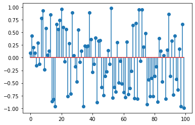
In theory, the signal \(x[n]\) extends to minus and plus infinity but for practical purposes, we represent it with a finite array as above.

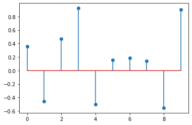
Now, let us create another random signal and embed it in \(x\).

# create another signal with random values: 
h = 2*(np.random.rand(10,)-0.5)
plt.figure(), plt.stem(h);

# embed it in x at location 19. The choice of 19 is arbitrary 
x[19:29] = h

# plot x again
plt.figure(),plt.stem(x);

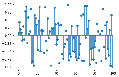
Now let us search for \(h\) in \(x\). It is a tedious task to do manually (by eye). Instead, we will simply apply cross-correlation operation to \(x\) and \(h\). The location with the highest response would give us the correct location:

y = np.correlate(x,h)
plt.stem(y)
print("location with highest response: ", np.argmax(y))

location with highest response:  19

Auto correlation

Auto-correlation operation of a continuous time signal \(x(t)\) is defined as

\[ y(t)= x(t)\star x(t)=\int_{-\infty}^{\infty}x^*(\tau)x(t+\tau)d\tau. \]

Similarly auto-correlation operation of a discrete time signal \(x[n]\) is defined as

\[ y[n]= x[n]\star x[n]=\sum_{k= -\infty}^{\infty}x^*[k]x[n+k]. \]

Auto-correlation measures the correlation of a signal with a lagged copy of itself as a function of the lag. It measures the similarity between different time instances of a function. This operation can be used to discover periodicities in signals and determine their periods as illustrated in the example below.

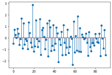
Suppose that we are given the following discrete time signal, and our task is to find out whether it presents periodicity and if so, its period.

x = np.array([-0.249, 1.012,-0.842, 0.287,-0.069,-0.248,-0.106, 0.125,-0.043, 0.028,
 -0.675,-0.166,-1.805, 0.135,-2.37 ,-0.272,-0.763,-0.005,-0.903,-0.395,
  1.682, 2.355, 0.439, 1.498, 1.854, 1.621,-1.151,-1.645,-1.575, 0.302,
 -2.179,-1.228, 0.491,-0.562, 0.22 ,-0.559, 0.906, 1.658,-0.567, 1.741,
  2.443, 1.582,-0.066, 1.14 ,-1.274,-0.584, 0.508,-1.536,-1.635,-2.063,
 -2.228, 0.017,-1.051,-0.532, 0.481,-0.563, 1.171,-0.06 , 1.191, 1.328,
 -0.751,-0.159, 0.326,-0.838,-2.18 ,-0.865,-0.501,-0.84 , 0.668,-0.101,
  1.2  ,-0.746,-0.432, 1.798, 0.682,-0.027, 2.123, 0.14 , 1.029, 0.6  ,
  0.726,-0.344,-0.162,-1.452,-1.645, 0.398,-0.739, 1.204, 0.656, 0.867,
 -0.382, 2.295, 0.849, 1.16 , 0.457,-0.343, 1.314,-0.031,-2.068,-0.475])
step = 0.28559933214452665
plt.stem(np.arange(0,100*step, step),x);
plt.xlabel('n');
plt.ylabel('x[n]');

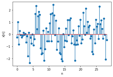
Note that this is a discrete time signal, therefore, it extends to minus and plus infinities. However, for practical reasons, we only show a part of it, representing it with a finite array, as shown above.

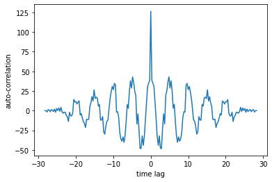
At first glance, it is not immediately clear whether the signal is periodic. To investigate this, we can apply the auto-correlation operation for analysis.

Remember, the auto-correlation operation measures the correlation of a signal with a lagged copy of itself as a function of the lag. Since the length of the given sequence is 100, the time indices for the lagged copy will run from -49 to +49. The auto-correlation result is given below.

y = np.correlate(x,x, mode='full')
plt.plot(np.linspace(-step*99,step*99,199), y);
plt.xlabel('time lag');
plt.ylabel('auto-correlation');

Let us zoom in to the positive time axis:

plt.plot(np.linspace(-step*99,step*99,199), y);
plt.xlabel('time lag');
plt.ylabel('auto-correlation');
plt.xlim((0,25));

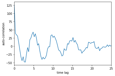
Do you notice the pattern? There are peaks at 0, 5, 10, 15, 20, i.e. at every time lag value of 5. This means that at every time lag value of 5, the correlation is high, which suggests overlapping parts of x and its time-lagged copy are very similar. From this observation, we can conclude that x might be periodic and the period is 5.

By the way, we should have plotted y using stem, however, a line plot (obtained by plot) better reveals the peaks.

In fact, here is the code we used to produce x:

n,step = np.linspace(0,9*np.pi, 100, retstep=True)
np.random.seed(1) # fixed for reproducibility
x = np.sin(n*(2*np.pi/5)) + 3*(np.random.rand(100,)-.5)
plt.stem(n, x);

# print(np.array2string(x, precision=3, separator=','))

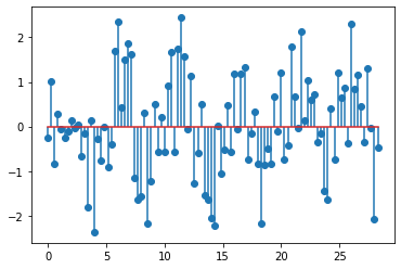
Indeed, the signal is \(x[n]=\sin(\frac{2\pi}{5} n)\), whose period is \(5\)!

---

Related content:

Explore convolution.

Explore convolution of two exponential functions.

A convolution (cross-correlation) example from machine learning.