Convolution

The convolution of two continuous time (CT) signals, \(x(t)\) and \(y(t)\), is defined as follows:

\[ z(t) = x(t) * y(t)= \int_{-\infty}^\infty x(\tau) y(t-\tau) d\tau. \]

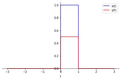
Let us see how convolution works step by step. We will use two rectangular pulse functions for ease of illustration. First, let us create these functions and plot them.

import sympy as sym

t = sym.symbols('t', real=True)

# define a pretty printing function
from IPython.display import display, Math, Latex
def print_latex(str, x):
    display(Math(str + "=" + sym.latex(x)))

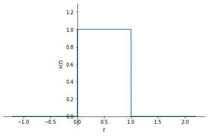
# define the first rectangular pulse. Width=1, height=1
x = sym.Piecewise( (0, t<0), (0, t>1), (1, True))
print_latex("x(t)", x)

# and plot it
sym.plot(x, (t, -1.2, 2.2), ylim=[-0.1, 1.3], ylabel=r'$x(t)$');


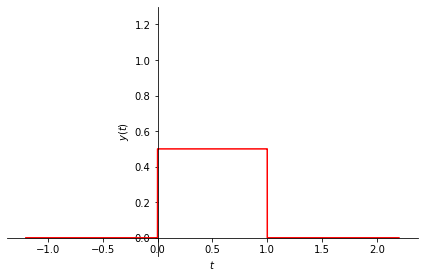
# define the second rectangular pulse. Width=1, height=0.5
y = sym.Piecewise( (0, t<-0), (0, t>1), (0.5, True))
print_latex("y(t)", y)

# and plot it
sym.plot(y, (t, -1.2, 2.2), ylim=[-0.1, 1.3], ylabel=r'$y(t)$', line_color='red');

\[\begin{split}\displaystyle x(t)=\begin{cases} 0 & \text{for}\: t > 1 \vee t < 0 \\1 & \text{otherwise} \end{cases}\end{split}\]

\[\begin{split}\displaystyle y(t)=\begin{cases} 0 & \text{for}\: t > 1 \vee t < 0 \\0.5 & \text{otherwise} \end{cases}\end{split}\]

Before showing intermediate steps, let us find out the solution and plot it. We can easily evaluate the convolution integral using Sympy’s integrate() function as shown below.

# variable of integration
tau = sym.symbols('tau', real=True)

# convolution integral
z = sym.integrate(x.subs(t, tau)*y.subs(t, t-tau), (tau, -sym.oo, sym.oo))
print_latex("z(t)",z)

sym.plot(z, (t, -1, 3),  ylabel=r'$z(t)$');

\[\displaystyle z(t)=0.5 \min\left(1, t\right) - 0.5 \min\left(1, t, \max\left(0, t - 1\right)\right)\]

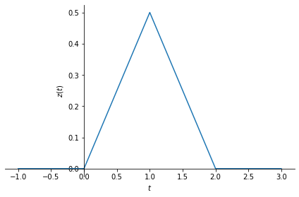
So, the result is a triangular pulse. Now let us understand how we obtained this result, step by step. First, let us implement a helper function to plot \(x(t)\) and \(y(t)\) on the same figure.

# plots t vs x and t vs y
def plot_xy(t, x,namex, y, namey):
    px = sym.plot(x, (t, -3, 3), legend=True, label=namex, ylabel="",
                  line_color='blue', show=False);
    py = sym.plot(y, (t, -3, 3), legend=True, label=namey, ylabel="",
                  line_color='red',  show=False);
    px.append(py[0])
    px.show();
    return px

plot_xy(t, x,"x(t)", y, "y(t)");

Let us now follow the steps given in Section 4.1.3 in the book.

Step 1

We would like to compute \(x(t)*y(t)\). The first step is to change the time variable \(t\) to the variable of integration \(\tau\). Now, instead of having \(x(t)\) and \(y(t)\), we have \(x(\tau)\) and \(y(\tau)\).

tau = sym.symbols('tau', real=True)

xtau = x.subs(t, tau)
ytau = y.subs(t, tau)

Step 2

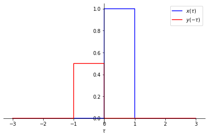
The second step is to time-reverse the second signal, i.e. in this case, \(y(\tau)\), to obtain \(y(-\tau)\). However, note that the convolution is commutative, that is, \(x(t)*y(t)\) is equivalent to \(y(t)*x(t)\).

plot_xy(tau, xtau, r'$x(\tau)$', ytau.subs(tau,-tau), r'$y(-\tau)$');

Step 3

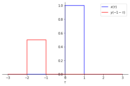
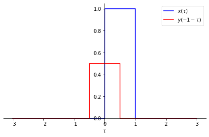
Now we shift \(y(-\tau)\) by \(t\), to obtain \(y(t-\tau)\). Below, you can see \(y(t-\tau)\) for different values of \(t\).

for t in [-1, 0.5, 2]:
    print("For t =", t)
    plot_xy(tau, xtau, r'$x(\tau)$', ytau.subs(tau,t-tau), r'$y(-1-\tau)$');

For t = -1

For t = 0.5

For t = 2

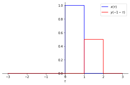
Step 4

Now let us take one of the values of \(t\) and compute the convolution integral. For example, for \(t=0.5\), the convolution integral is

\[ z(0.5) = \int_{-\infty}^\infty x(\tau) y(0.5-\tau) d\tau. \]

This expression calculates the integral of the multiplication of two functions, which corresponds to the area under \(y(t-\tau)\) weighted by \(x(\tau)\). This area is marked with yellow color below.

import numpy as np
t=.5
print("For t =",t)
p1 = sym.plot(xtau, (tau, -2, 2), show=False)
p2 = sym.plot(ytau.subs(tau,t-tau), (tau, -2, 2), show=False)
xarray = np.linspace(-2, 2, 500)

xval = np.array([xtau.subs(tau, val) for val in xarray], dtype=float)
yval = np.array([ytau.subs(tau, t-val) for val in xarray], dtype=float)

#yarray = np.min(xtau.eval(xarray), ytau.subs(tau,t-tau).eval(xarray))
p3 = sym.plot(fill={'x':xarray, 'y1': np.minimum(xval,yval), 'edgecolor':'none', 
                                      'facecolor':'yellow'}, show=False)
p3.append(p1[0])
p3.append(p2[0])
p3.show()

For t = 0.5

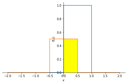
You can change the value of \(t\) above to see how the yellow area changes.

Animation of the whole process

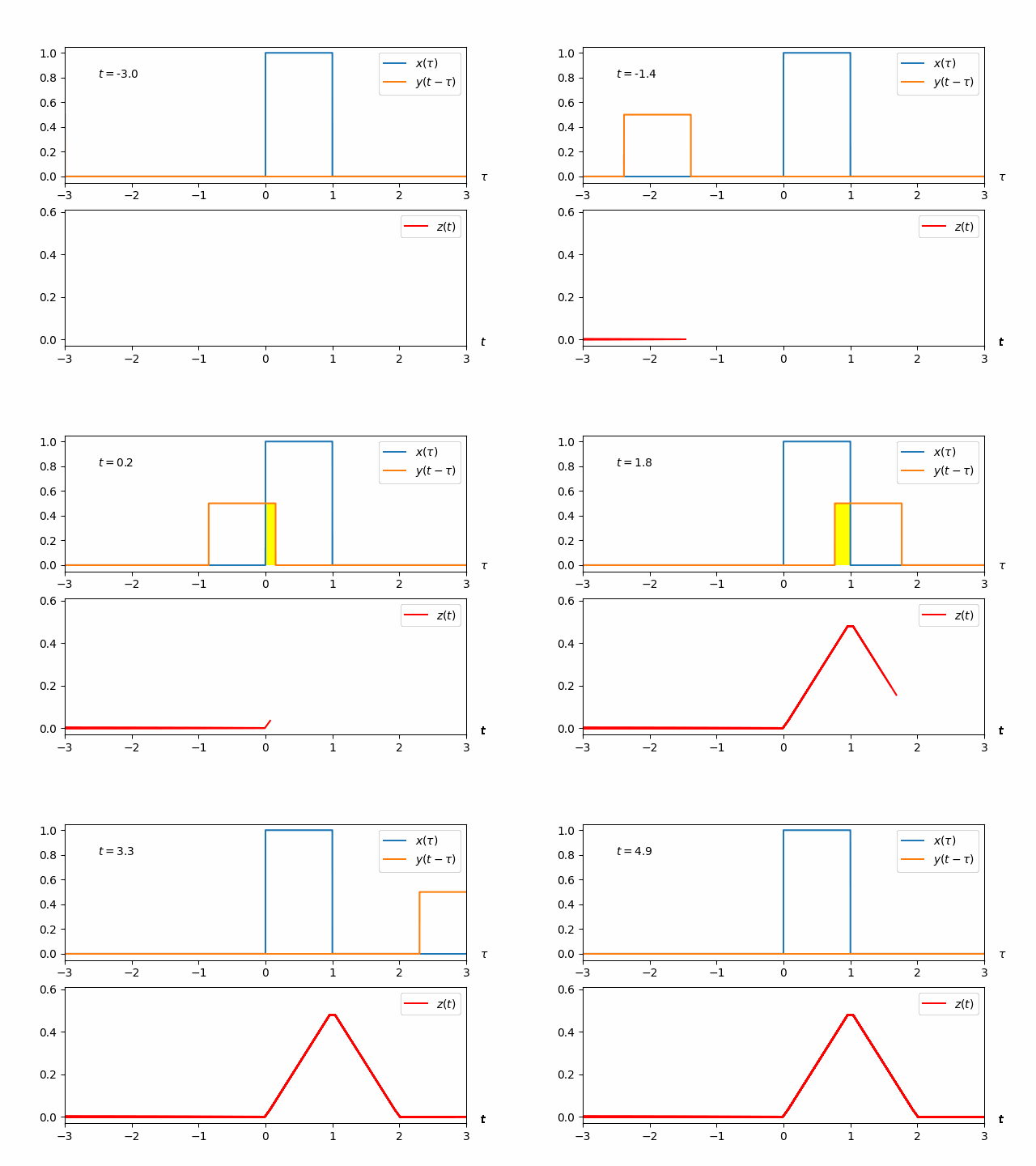
The whole process of convoluting \(x(t)\) with \(y(t)\), that is, computing

\[ z(t) = x(t) * y(t)= \int_{-\infty}^\infty x(\tau) y(t-\tau) d\tau, \]

is shown in the animation below. The code that produced this animation follows.

from matplotlib import pyplot as plt
import matplotlib.animation as animation

ts=np.linspace(-3, 5, 100)
z = np.zeros(len(ts))

fig, axs = plt.subplots(2)

def animate(i): 
    t = ts[i]

    p1 = sym.plot(xtau, (tau, -3, 3), line_color='blue', show=False)
    p1x,p1y = p1[0].get_data()

    p2 = sym.plot(ytau.subs(tau,t-tau), (tau, -3, 3), line_color='orange', 
                    show=False)
    p2x,p2y = p2[0].get_data()

    z[i] = sym.integrate(xtau*ytau.subs(tau, t-tau), (tau, -sym.oo, sym.oo))

    # for area under the curve
    xarray = np.linspace(-3, 3, 500)
    xval = np.array([xtau.subs(tau, val) for val in xarray], dtype=float)
    yval = np.array([ytau.subs(tau, t-val) for val in xarray], dtype=float)

    axs[0].cla()
    axs[0].set_xlim((-3,3))
    axs[0].text(3.2,-.03,r'$\tau$')
    axs[0].text(-2.5,.8,r'$t=$'+f'{t:.1f}')
    
    axs[0].plot(p1x,p1y, p2x, p2y) 
    axs[0].legend([r'$x(\tau)$',r'$y(t-\tau)$'])
    axs[0].fill_between(xarray, np.minimum(xval, yval), color='yellow', edgecolor='none')

    axs[1].set_xlim((-3,3))    
    axs[1].set_ylim((-.03,.61))
    axs[1].text(3.2,-.03,r'$t$')
    axs[1].plot(ts[0:i], z[0:i],color='red')
    axs[1].legend([r'$z(t)$'])

ani = animation.FuncAnimation(fig, animate, repeat=True,
                                    frames=len(ts) - 1, interval=50)

# #To save the animation as a gif file: 
# writer = animation.PillowWriter(fps=4,
#                                 metadata=dict(artist='384book'),
#                                 bitrate=1800)
# ani.save('conv_animation.gif', writer=writer)
plt.close()

Convolution and LTI systems

The convolution integral uniquely identifies a linear, time-invariant (LTI) system. Formally, let \(x(t)\) be the input to the system and \(h(t)\) represent the impulse response of the system, then the output \(y(t)\) can be computed using the convolution integral:

\[ y(t) = x(t) * h(t)= \int_{-\infty}^\infty x(\tau) h(t-\tau) d\tau. \]

Example: Consider an LTI system whose impulse response is \(h(t)=\delta(t-2)\). What would be the output of this system when the input is \(x(t)\)?

The answer is

\[ y(t) = x(t) * \delta(t-2)= \int_{-\infty}^\infty x(\tau) \delta(t-\tau-2) d\tau = x(t-2). \]

You can easily verify this answer using Sympy:

# time variable
t = sym.symbols('t', real=True)

# variable of integration
tau = sym.symbols('tau', real=True)

# input
x = sym.Function('x')(t)

# impulse response
delta = sym.DiracDelta(t)
h = delta.subs(t, t-2)

# convolution integral
y = sym.integrate(x.subs(t, tau)*h.subs(t, t-tau), (tau, -sym.oo, sym.oo))
y

\[\displaystyle x{\left(t - 2 \right)}\]

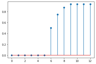
Another example: Let us find the output of a discrete time LTI system whose impulse response is \(h[n]=0.5^n u[n]\), when the input is \(x[n]=u[n]\).

For discrete time signals and systems, it is more convenient to use numpy. However, both \(x[n]\) and \(h[n]\) extend to infinity and it is challenging to both represent them and compute their convolution for the whole time axis. Instead, we will represent some finite parts of \(x[n]\) and \(h[n]\) with finite numpy arrays and compute their “valid” convolution to avoid boundary effects. Below you can find a piece of code that carries out this task.

import numpy as np
from matplotlib import pyplot as plt
# input
x = np.array([0,0,0,0,0,0,0,0,0,1,1,1,1,1,1,1,1,1,1], dtype=float)

# impulse response of the system
h = np.array([0,0,0,0.5,0.5**2, 0.5**3, 0.5**4], dtype=float)

# the output y
y = np.convolve(x,h,'valid')
y

plt.stem(y);

---

Related content:

Explore convolution of two exponential functions.

Explore cross-correlation and auto-correlation.

A convolution (cross-correlation) example from machine learning.