Operations on the Time Variable of Signals

Operations on the Time Variable of Signals#

Previously, we have seen elementary operations on a signal. Here we will study how the signal changes when we apply elementary operations on the independent variable, that is the time variable.

Time shift#

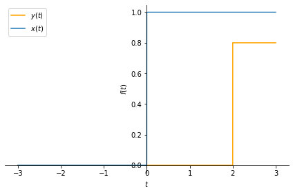
Time shift operation for a continuous time signal replaces the time variable $t$ of $x (t)$ by $t^{'} = (t - T)$ to obtain $x (t^{'}) = x (t - T)$ , where $T$ is the amount of shift.

Let us see the effect of this operation on a unit step signal, also called as the Heaviside step function (after Oliver Heaviside).

import sympy as sym
sym.init_printing()

t = sym.symbols('t', real=True)

# amount of time shift:
T = 2 

# original signal. this corresponds to $u(t)$ in our book 
x = sym.Heaviside(t)

# new, time-shifted signal:
y = 0.8*x.subs(t, t-T)  # we also scaled the signal (by 0.8) so that 
                        # both x and y are visible in the plot. 

# plot
px = sym.plot(x, (t, -3, 3), legend=True, label='$x(t)$', show=False);
py = sym.plot(y, (t, -3, 3), legend=True, label=r'$y(t)$', show=False, 
              line_color='orange')
py.extend(px)
py.show()

_images/b46d20e8ab61ce77d13be875b0144db5c477199f6a97704bac80a1051b223731.png

Note: The subs(a,b) operation in SymPy basically replaces all occurences of expression a with expression b, symbolically. This capability offers us an elegant way of manipulating the time variable of signals.

Exercise: Change the values of $T$ above and see its effect.

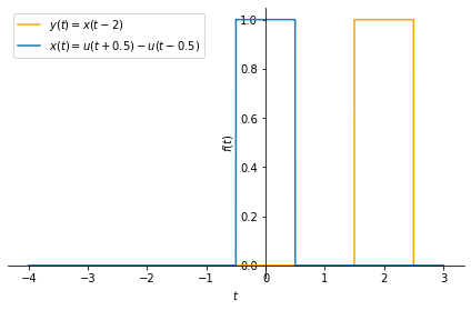
Let us look at another example, this time with a rectangular pulse signal:

# we obtain a rectangular pulse signal as a difference of two, time-shifted 
# unit step signals: 
x = sym.Heaviside(t + 1/2) - sym.Heaviside(t - 1/2)

# let us now apply time shift: 
y = x.subs(t, t-2)

# plot
px = sym.plot(x, (t, -4, 3), legend=True, label='$x(t)=u(t+0.5)-u(t-0.5)$', 
              show=False);
py = sym.plot(y, (t, -4, 3), legend=True, label=r'$y(t)=x(t-2)$', show=False, 
              line_color='orange')
py.extend(px)
py.show()

_images/b4abf9b1211969e51f06454e7f59b05f0c22893d2202993fddf99cb4641c247a.png

Exercise: write code to explore the time-shift operation for discrete-time signals.

Time reverse#

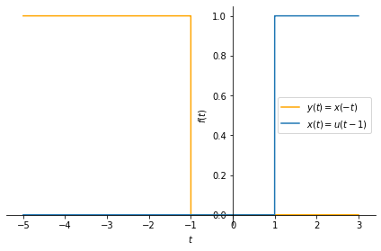
Time reverse operation of a continuous time signal changes the sign of the time variable $t$ of the signal, $x (t)$ , by $t^{'} = - t$ to obtain $x (t^{'}) = x (- t)$ . This opertation basically flips the signal along the horizontal axis. Let us see its effect on a unit step signal:

# let us define a unit step signal: 
x = sym.Heaviside(t-1)

# let us now apply time reverse: 
y = x.subs(t, -t)

# plot
px = sym.plot(x, (t, -5, 3), legend=True, label='$x(t)=u(t-1)$', 
              show=False);
py = sym.plot(y, (t, -5, 3), legend=True, label=r'$y(t)=x(-t)$', show=False, 
              line_color='orange')
py.extend(px)
py.show()

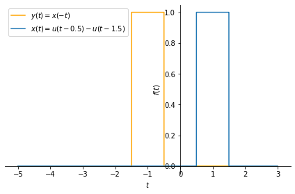
_images/ad88d83b080488b1f875a61e88aabbc48bc5985d33a353119b70967789f5bdfc.png

Let us look at another example, this time with a rectangular pulse:

# let us start with a time-shifted rectangular pulse: 
x = sym.Heaviside(t-0.5) - sym.Heaviside(t - 1.5)

# let us now apply time reverse: 
y = x.subs(t, -t)

# plot
px = sym.plot(x, (t, -5, 3), legend=True, label='$x(t)=u(t-0.5)-u(t-1.5)$', 
              show=False);
py = sym.plot(y, (t, -5, 3), legend=True, label=r'$y(t)=x(-t)$', show=False, 
              line_color='orange')
py.extend(px)
py.show()

_images/3019e354bd6523b00addf2db9a6a573ef64e679e4ab68e38433ce6cf9a9beaea.png

Time scale#

Time scale operation of a continuous time function replaces the time variable, $t$ of $x (t)$ by $t^{'} = a t$ to obtain $x (t^{'}) = x (a t)$ , where $a$ is a time scale parameter.

Let us apply it to a periodic continuous time signal:

a = 1.5

x = sym.cos(t)
y = x.subs(t,a*t)

# plot
px = sym.plot(x, (t, -10, 10), legend=True, label='$x(t)=cos(t)$', show=False);
py = sym.plot(y, (t, -10, 10), legend=True, label=r'$y(t)=x(0.5t)$', show=False, 
              line_color='orange')
py.extend(px)
py.show()

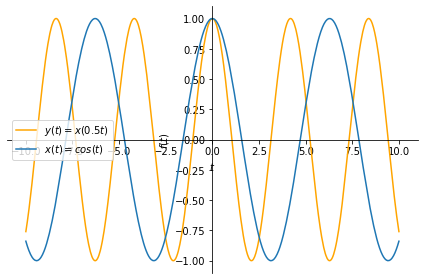
_images/fba059b4d8363a3f388398a477271208e31d521bc16fd5e0f4f710935e43a5b5.png

Play with the value of a above. As you will see, values larger than $1$ squeezes the signal, whereas values less than $1$ (and greater than $0$ ) stretches the signal.

Also,note that the time reverse operation is a special case of time scaling where $a = - 1$ .

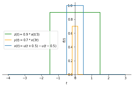
Let us look at another example below. Here we will apply time scaling to a rectangular pulse.

# rectangular pulse: 
x = sym.Heaviside(t + 1/2) - sym.Heaviside(t - 1/2)

# let us now apply time scaling: 
a = 3
y = 0.7*x.subs(t, a*t) # we scale the signal so that it can be seen better

# another one: 
b = 1/3
z = 0.9*x.subs(t, b*t) 

# plot
px = sym.plot(x, (t, -4, 3), legend=True, label='$x(t)=u(t+0.5)-u(t-0.5)$', 
              show=False);
py = sym.plot(y, (t, -4, 3), legend=True, label=r'$y(t)=0.7*x(3t)$', show=False, 
              line_color='orange')
pz = sym.plot(z, (t, -4, 3), legend=True, label=r'$z(t)=0.9*x(t/3)$', show=False, 
              line_color='green')
pz.extend(py)
pz.extend(px)
pz.show()

_images/b3456a535ae3e4945875b8389da9dbad6a0d63a3169c6754c2cef4c2e75ac4bf.png

Time scale and shift#

We can apply time scale and time shift operations simultaneously to obtain $x (a t + b)$ from $x (t)$ .

An example follows.

# let us create a rectangular pulse: 
rect = sym.Heaviside(t + 1/2) - sym.Heaviside(t - 1/2)

# then, let's create another signal as a combination of two rectangular pulses: 
x = rect + 2*rect.subs(t, t-1)

# time scale & shift applied together: 
a = 4
b = 5
y = x.subs(t, a*t+b)

# plot
px = sym.plot(x, (t, -3, 3), legend=True, label='$x(t)$', show=False);
py = sym.plot(y, (t, -3, 3), legend=True, label=r'$y(t)$', show=False, 
              line_color='orange')
py.extend(px)
py.show()

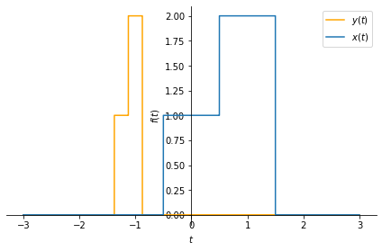
_images/314afaf272e68259757a04e0b7138e9d81870518b804e504fb2b963e8b4c049a.png

Notice how the signal $x (t)$ gets squeezed and shifted at the same time. Play with the values a and b and see their effect. We especially encourage to try negative values for a to obtain a time reverse effect.

Finally, let us look at an example where we apply time scale and shift operations to a discrete time signal.

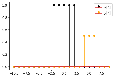
In discrete time signals, the time (independent) variable is by definition an integer. And, when we apply time scaling, the time variable might become a non-integer number. For such cases, it is conventional to set the value of the signal to zero. One possible implementation to achieve this is given below.

import numpy as np 
from matplotlib import pyplot as plt

# define the time variable. 
n = np.arange(-10,10, 1.0)

# define signal x[n]
def x(n):
    # if the time variable is not an integer, return 0
    if not n==np.rint(n):
        print("argument not integer!")
        return 0
    
    return 1*np.logical_and(n>=-2,n<=2)

# the function above takes a scalar. for it to work on a vector of elements, we
# should vectorize is: 
vx = np.vectorize(x)

# apply time scale and shift to x[n] to obtain a new signal 
# y[n] = 0.5*x[0.5*(n-2)]
def y(n): 
    a = 0.5
    b = -3
    return .5*vx(a*(n+b))

plt.stem(n, vx(n), linefmt='black')
plt.stem(n, y(n), linefmt='orange');

plt.legend((r'$x[n]$', r'$y[n]$'));

argument not integer!
argument not integer!
argument not integer!
argument not integer!
argument not integer!
argument not integer!
argument not integer!
argument not integer!
argument not integer!
argument not integer!
argument not integer!

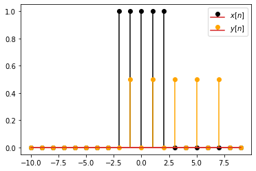
_images/5014b0026453f3a939afc79fa48882dc71a2eb00ab2a5396c1c1110eaa98a860.png

Here we scaled the value of $y [n]$ by $0.5$ , so that both signals are visible.

Try different values for a and b above, which define the new signal $y [n]$ .

For $| a | < 1$ , the signal is expanded by inserting zero values in between the time instances of the original signal. This opetation is called expansion.

For $| a | > 1$ , the signal is squeezed by discarding the samples of the original signal between $a n$ and $a (n - 1)$ time instances, for all $n$ . This operation is called decimation. You can obtain an example for decimation by setting a larger than 1 above.

# apply time scale and shift to x[n] to obtain a new signal 
def y(n): 
    a = 2
    b = -5
    return .5*vx(a*(n+b))

plt.stem(n, vx(n), linefmt='black')
plt.stem(n, y(n), linefmt='orange');

plt.legend((r'$x[n]$', r'$y[n]$'));

_images/4c9fffb7b2670a3d36cbe66259b101ec600441f190d1ed4a5494c4081161884a.png