Types of signals#
We represent signals using mathematical functions. A function maps elements in a domain set to the elements in a range set. Throughout this book, we will mostly deal with functions of a single independent variable, which usually represents time, denoted with \(t\) or \(n\).
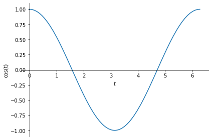
Let us create the following signal using SymPy and plot it:
\(x(t) = \cos(t)\).
First, we need to define the independent variable, that is time, represented by the variable \(t\):
import sympy as sym

t = sym.symbols('t', real=True)
We defined \(t\) to be a variable taking values from real numbers by saying
real=True. Let us now create a signal that depends on \(t\), and
plot it. Remember, a signal is a function.
# the signal:
x = sym.cos(t)

sym.plot(x, (t, 0, 2*sym.pi), ylabel='cos(t)');
Notes:
The
sym.plot()call produces one line of text output, which is not useful for our purposes here. So, we supress it using a semicolon at the end ofsym.plot(). You can try removing it and see the useless text output yourself.The
(t, 0, 2*sym.pi)argument limits the x-axis, i.e. the \(t\) variable, to \([0,2\pi]\) for the purposes of plotting. The signal continues to exist beyond this interval, towards \(-\infty\) and \(\infty\).The
ylabel='cos(t)'argument prints a label for the y-axis.
In Section 1.3.2 of our book, we describe there types of signals:
continuous time (CT) signals,
discrete time (DT) signals and
digital signals.
In the following, we will define and plot example signals for each category.
Continuous time (CT) signals#
Continuous time (CT) signals are represented by continuous functions, where both the
domain and the range consists of real numbers. It is conventional to use the
symbol t as the continuous domain variable. The example signal above, i.e.
\(x(t) = \cos(t)\), is a CT signal.
Let us define and plot another CT signal, e.g. \(x(t) = e^{-t}\).
x = sym.exp(-t)

sym.plot(x, (t,0,5), ylabel='$e^{-t}$');
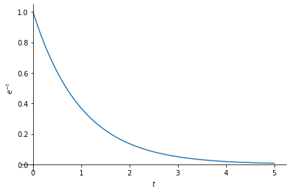
Note that we limited \(t\) to the interval \([0,5]\) for plotting purposes. The signal extends to \(-\infty\) and \(\infty\).
Discrete time (DT) signals#
Discrete time signals are represented by discrete functions, where the domain variable is an integer and the range is a real number. It is conventional to use the symbol \(n\) as the discrete domain variable, representing integers.
Let us define and plot the following DT signal:
\(x[n]=e^{-n}\).
import numpy as np
import matplotlib.pyplot as plt

n = np.arange(-2, 3)
x = np.exp(-n)

plt.stem(n,x);
plt.xlabel('$n$')
plt.ylabel('$e^{-n}$')
Text(0, 0.5, '$e^{-n}$')
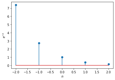
Note that we limited \(n\) to the interval \([-2,2]\) for plotting purposes. The signal extends to \(-\infty\) and \(\infty\).
Digital signals#
Digital signals are represented by range-quantized discrete functions. Both the domain and range of the digital signals consist of integer numbers.
Suppose that we have a thermometer which can provide its temperature measurement only in integer numbers. If we record values from this thermometer at regular intervals of time, then we would obtain a digital signal.
Let us define an example digital signal as follows:
\(x[n]=\begin{cases} 0, & n<-3, \\ 2, & -3 \le n < -1, \\ 1, & -1 \le n < 1, \\ 3, & 1 \le n < 3, \\ 0, & n \ge 3 \end{cases}\)
where both \(n\) and \(x[n]\) are integers.
n = np.arange(-5, 6)
x = [0,0,2,2,1,1,3,3,0,0,0]

plt.stem(n,x);
plt.xlabel('$n$')
plt.ylabel('$x[n]$')
Text(0, 0.5, '$x[n]$')
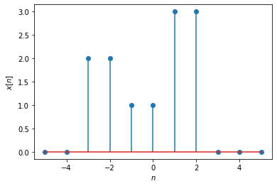
Note that we limited \(n\) to the interval \([-5,5]\) for plotting purposes. The signal extends to \(-\infty\) and \(\infty\).
Exercise: Define and plot CT, DT and digital signals (different than above) on your own.
Related content:
Explore elementary operations on signals.
