Elementary operations on signals#
Here we will explore addition and scaling operations on signals.
Consider the following CT signal:
\(x(t)=\cos(t)\).
You can add a constant b to this signal. Let us see the effect of this
operation by plotting the new signal:
\(y(t)=x(t)+b=\cos(t)+b\).
import sympy as sym

t = sym.symbols('t', real=True)

# scalar constant
b = 1

# the signals:
x = sym.cos(t)
y = sym.cos(t)+b

p1 = sym.plot(x, (t, 0, 2*sym.pi), legend=True, label='cos(t)', show=False);
p2 = sym.plot(y, (t, 0, 2*sym.pi), legend=True, label='cos(t)+b', show=False);

p1.append(p2[0])
p1.show()
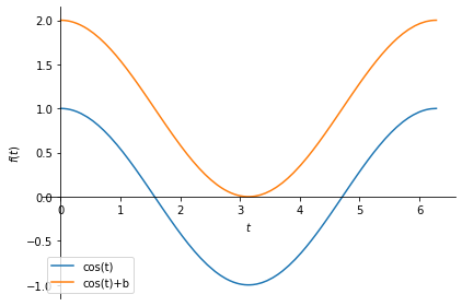
Change the value of constant b above to see its effect.
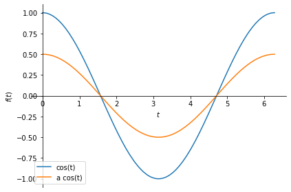
When you multiply a signal with a scalar number, the value of the signal scales accordingly. Observe the plots of \(x(t)\) and \(y(t)\) below.
# scalar constant
a = 0.5

# the signal:
x = sym.cos(t)
y = a*sym.cos(t)

p1 = sym.plot(x, (t, 0, 2*sym.pi), legend=True, label='cos(t)', show=False);
p2 = sym.plot(y, (t, 0, 2*sym.pi), legend=True, label='a cos(t)', show=False);

p1.append(p2[0])
p1.show()
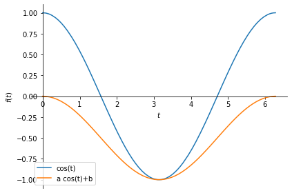
You can combine both operations to obtain:
\(y(t) = a x(t) + b\).
Change the values of a and b below to see their effects.
# scalar constant
a = 0.5
b = -0.5

# the signal:
x = sym.cos(t)
y = a*sym.cos(t)+b

p1 = sym.plot(x, (t, 0, 2*sym.pi), legend=True, label='cos(t)', show=False);
p2 = sym.plot(y, (t, 0, 2*sym.pi), legend=True, label='a cos(t)+b', show=False);

p1.append(p2[0])
p1.show()
We can also add two or more signals together to obtain a more complicated signal.
Let us now create two signals, \(x\) and \(y\), and add them to obtain a third signal, \(z\). Let
\(x(t) = \cos(t) -\frac{1}{2}\),
\(y(t) = \frac{1}{5} t \), and
\(z(t) = x(t) + y(t)\).
The following code creates \(z(t)\) and plots it.
x = sym.cos(t)-0.5
y = 0.2*t
z = x + y

sym.plot(z);
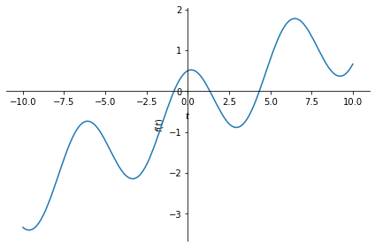
Exercise: Play with the coefficients of \(x\), \(y\), and \(t\) above. Observe how the shape of \(z(t)\) changes.
Related content:
Explore different types of signals.