Sampling and reconstruction of a discrete time signal

Sampling and reconstruction of a discrete time signal#

Sampling and reconstruction of a discrete time signal is very similar to that of a continuous time signal, which was descibed before.

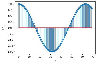
Let us create a discrete time signal x[n] and plot it:

import numpy as np
from matplotlib import pyplot as plt

ns = np.arange(0,70,1)

w0 = 0.1

def x(n):
    return np.cos(w0*n)

plt.stem(ns, x(ns))
plt.ylabel(r'$x[n]$')
plt.xlabel(r'$n$');

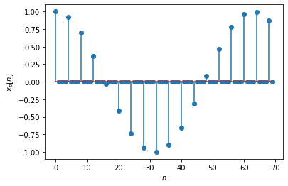
_images/6dd0933cc4e97033aab507cd789265c43f07b5dc26f91ff7eee3293b23f0d159.png

Let us now sample this signal using a sampling period of \(N=4\):

N = 4

def xp(n):
    return (n%N ==0)*x(n)

The sampled signal looks like this:

plt.stem(xp(ns))
plt.ylabel(r'$x_p[n]$')
plt.xlabel(r'$n$');

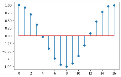
_images/dd097e578abc541552b172ce2b43ca1ce48e24440dbae666dfd69a64d63d3446.png

Notice the zeros in between the sampled values. We can get rid of those zero values by decimating the signal, that is, by keeping every \(N\) element. Here is the decimated signal \(x_b[n]=x_p[nN]\):

xb = xp(ns[:int(len(ns)/N)]*N)
plt.stem(xb);

_images/d9c089e77deade9cb5c8080cb9b77595c2f5f6c4e28478295851824f5306f726.png

Now we can reconstruct back the original signal \(x[n]\) from \(x_b[n]\), which is equivalent to \(x_p[nN]\):

ks = np.arange(-100,100,1)

# sampling frequency
ws = 2*np.pi/N  

def xr(n):
    return sum(xp(k*N)*(1/N)*np.sinc((n-k*N)/N) for k in ks)

qq=xr(np.arange(1,70,1))
plt.stem(qq)
plt.ylabel(r'$x_r[n]$')
plt.xlabel(r'$n$');

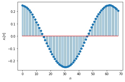
_images/21993b03ca59b977d25fafe1cc1ad47e2800f6d715f1bf9c1e4a9460bf123ca0.png

Here, we used the fact that passing the signal through an ideal low-pass filter \(H(j \omega)\) is equivalent to convolving the signal with a \(\text{sinc}(\dot)\) function.