Sampling and reconstruction of a continuous time signal

In this notebook, we will explore how the impulse train sampling and reconstruction of a continuous time signal works. The sampling and reconstruction pipeline is illustrated below.

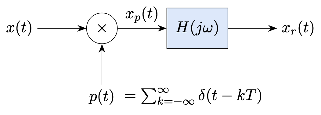
Here \(x(t)\) is the CT input signal to be sampled and reconstructed, and \(x_r(t)\) is the reconstruction result. \(p(t)\) represents an impulse train and \(x_p(t)\) is the samples of \(x(t)\). \(x_r(t)\) is obtained by low-pass filtering the sampled signal \(x_p(t)\). The implementation of these steps, especially sampling a signal with a series of Dirac delta impulses that extend to minus and plus infinities and integrals involving such unlimited signals, is not straigthforward and one do not always get the expected results. However, fortunately, we can implement all these sampling and reconstruction steps while staying totally in time domain, as we explain below.

Sampling

Sampling basically corresponds to multiplying \(x(t)\) with \(p(t)= \sum_{n=-\infty}^\infty \delta(t-nT)\):

\[ x_p(t) = \sum_{n=-\infty}^\infty x(nT) \delta(t-nT), \]

where \(T\) is the sampling period. The sampling period \(\omega_s\) is related to \(T\) as \(\omega_s = \frac{2\pi}{T}\).

At the end of this process, we have sampled values \(x(nT)\) for integer \(n=-\infty \dots \infty\), and the sampling period \(T\), or equivalently, the sampling frequency \(\omega_s\). The original signal \(x(t)\) can be reconstructed using these two information as shown in the following.

Reconstruction

The reconstructed signal, \(x_r(t)\), is the result of convolving \(x_p(t)\) with an ideal low-pass filter, whose impulse response is denoted with \(h(t)\):

\[\begin{split} \begin{aligned} x_r(t) & = x_p(t)*h(t) = \int_{-\infty}^\infty x_p(\tau) h(t-\tau) d\tau \\ & = \int_{-\infty}^\infty \sum_{n=-\infty}^\infty x(\tau = nT) \delta(t-\tau) h(t-\tau) d\tau \end{aligned}. \end{split}\]

Remember the properties of the Dirac delta: it is non-zero only at \(t=\tau\) and its integral is equal to 1. Due to these properties, we have

\[ x_r(t) = \sum_{n=-\infty}^\infty x(nT) h(t-nT). \]

The ideal low-pass filter for the reconstruction is

\[\begin{split} H(j\omega) = \begin{cases} T, & |\omega|< \frac{\omega_s}{2} \\ 0, & \text{otherwise.} \end{cases} \end{split}\]

We can find out the impulse response \(h(t)\) of this filter using the Fourier transform table (Table 8.2):

\[ h(t) = \frac{T \sin(\frac{\omega_s}{2}t)}{\pi t}, \]

which is basically a sinc function scaled by the sampling period \(T\).

An example

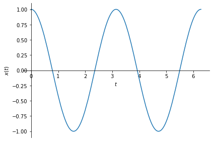
Now let us apply the sampling and reconstruction process described above to a simple periodic cosine signal: \(x(t) = \cos(\omega_0 t)\).

import sympy as sym

t = sym.symbols('t', real=True)

w0 = 2
x = sym.cos(w0*t)

sym.plot(x, (t, 0, 2*sym.pi), ylabel=r'$x(t)$');

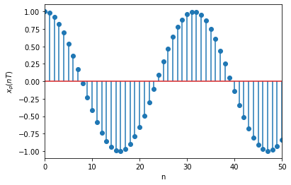
Let us now sample this signal with sampling period \(T=0.1\), that is, with sampling frequency \(\omega_s = \frac{2\pi}{0.1}=20\pi\).

# sampling period 
T = 0.1
n = sym.symbols('n', integer=True)

# we create a temporary function f, which we will call to get values of x_p
f = sym.Lambda(n, x.subs(t, n*T))

import numpy as np

# here we sample the signal for integer n values from -100 to 100.
# Theoretically, we should do the sampling from minus infinity to plus infinity
# but for practical reasons, we limit this. 
ns = np.arange(-100,100)
xp = [f(i) for i in ns]

The sampled values can be plotted as follows:

import matplotlib.pyplot as plt
plt.stem(ns,xp)
plt.xlim([0,50])
plt.xlabel('n')
plt.ylabel(r'$x_p(nT)$');

Now we can reconstruct back \(x\) usingxp and T:

xr = sum(xp[i]*T*sym.sin((t-ns[i]*T)*sym.pi/T)/(sym.pi*(t-ns[i]*T)) for i in ns)
sym.plot(xr, (t, 0, 2*sym.pi), ylabel=r'$x_r(t)$');

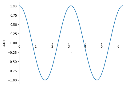
Note that \(x_r(t)\) is basically the same signal as \(x(t)\). Here is \(x(t)\)’s plot:

sym.plot(x, (t, 0, 2*sym.pi), ylabel=r'$x(t)$');

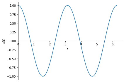
So, our sampling and reconstruction worked! It worked because our sampling frequency conformed with the Nyquist rate:

\[ \omega_s > 2\omega_M, \]

where \(2\omega_M\) is the bandwidth of the input signal. In our case, this bandwidth is \(2\omega_0=4\). And the sampling frequency was \(\omega_s=20\pi\).

Now let us try the same procedure with another sampling period, this time let us use a sampling frequency less than the bandwidth of the signal. For example, \(\omega_s = \pi\), which corresponds to \(T = \frac{2\pi}{\omega_s} = 2\).

# sampling: 
T = 2
f = sym.Lambda(n, x.subs(t, n*T))
xp = [f(i) for i in ns]

# reconstruction:
xr = sum(xp[i]*T*sym.sin((t-ns[i]*T)*sym.pi/T)/(sym.pi*(t-ns[i]*T)) for i in ns)
sym.plot(xr, (t, 0, 2*sym.pi), ylabel=r'$x_r(t)$');
sym.plot(x, (t, 0, 2*sym.pi),  ylabel=r'$x(t)$');

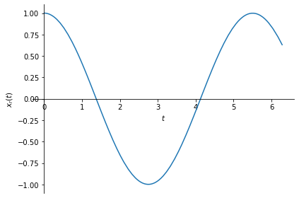
As you can see above, \(x_r(t)\) and \(x(t)\) are not the same signals. This happened because our sampling rate did not obey the Nyquist rate. Or, in other words, we undersampled the signal, or, aliasing occured.

You are encouraged to reproduce the sampling and reconstruction procedure above for another signal and sampling period of your choice.

---

Related content:

Sampling and reconstruction with first-order hold.

Sampling and reconstruction of a discrete time signal.