Sampling and reconstruction with first-order hold#
The impulse train sampling and reconstruction described in our pprevious notebook](in1101) is ideal for teaching how sampling and reconstruction work. However, in practice, it is not possible to realize zero-width, infinite-height impulses. First order hold sampling, also called linear interpolation, offers a practical method for sampling a continuous time signal in time domain.
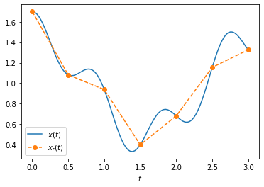
It basically corresponds to connecting the dots, where dots are sampled values. An example is provided in the plot below.
import numpy as np
from matplotlib import pyplot as plt

def x(t):
    return np.cos(0.1*t) + 0.5*np.cos(2*t) + 0.2*np.cos(7*t)

ts = np.linspace(0, 3, 100)
xs = [x(t) for t in ts]

plt.plot(ts, xs, label=r'$x(t)$')

ns = np.arange(0,3.1,.5)
plt.plot(ns, [x(t) for t in ns], 'o--', label=r'$x_r(t)$')
plt.xlabel(r'$t$')
plt.legend();
The question is how can we obtain \(x_r(t)\) from \(x(t)\) mathematically?
We can use the usual sampling and reconstruction pipeline:
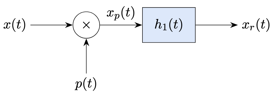
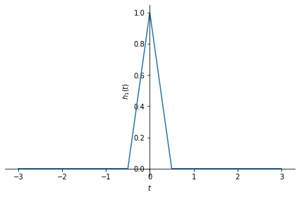
What should be the impulse response \(h_1(t)\)? To linearly interpolate between sampled points, the contribution of a point should be maximum at the location of the point itself and it should linearly decrease as you move away from the point. Such an effect is obtained by a triangular impulse response:
import sympy as sym

t,T = sym.symbols('t T', real=True)
T = 0.5 # sampling period
h = sym.Piecewise( (0, t<-T), ((T+t)/T, t<0), ((T-t)/T, t<T), (0, True))
sym.plot(h, (t, -3,3), ylabel=r'$h_1(t)$');
Below, we do the sampling:
# the signal
x = sym.cos(0.1*t) + 0.5*sym.cos(2*t) + 0.2*sym.cos(7*t)

# sampling period
T = 0.5
n = sym.symbols('n', integer=True)

# we create a temporary function f, which we will call to get values of x_p
f = sym.Lambda(n, x.subs(t, n*T))

import numpy as np

# here we sample the signal for integer n values from -100 to 100.
# Theoretically, we should do the sampling from minus infinity to plus infinity
# but for practical reasons, we limit this.
ns = np.arange(-100,100)
xp = [f(i) for i in ns]
And, then reconstruction, which is simply convolving \(x_p(t)\) with \(h_1(t)\):
# interpolation filter, h1(t)
h = sym.Piecewise( (0, t<-T), ((T+t)/T, t<0), ((T-t)/T, t<T), (0, True))

# reconstruction
xr = sum(x.subs(t,ns[i]*T) * h.subs(t, t-ns[i]*T) for i in ns)
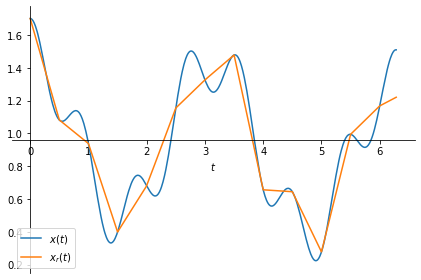
When we plot \(x(t)\) and \(x_r(t)\), we observe that \(x_r(t)\) linearly interpolates \(x(t)\) with sampling period \(T=0.5\).
p1 = sym.plot(xr, (t, 0, 2*sym.pi), label=r'$x_r(t)$', ylabel='', legend=True, show=False);
p2 = sym.plot(x, (t, 0, 2*sym.pi), label=r'$x(t)$', ylabel='', legend=True, show=False)
p2.extend(p1)
p2.show()
Related content: