Trigonometric Fourier series representation

Trigonometric Fourier series representation#

In Section 6.9 of the book, we introduces the trigonometric Fourier series.

SymPy has a native function to compute trigonometric Fourier series. However, it uses a slightly different notation.

SymPy analyses the given signal in a finite period as opposed to the whole real axis (from minus infinity to plus infinity) as we did in the book.

In SymPy, the Fourier trigonometric series of \(x(t)\) over the interval \((l,u)\) is defined as

\[ x(t) = \frac{a_0}{2} + \sum_{n=1}^{\infty} \left( a_n \cos(\frac{2n\pi t}{u-l}) + b_n \sin(\frac{2n\pi t}{u-l}) \right) \]

where the coefficients are as follows:

\[ a_0 = \frac{2}{u-l} \int_l^u x(t) dt, \]

\[ a_n = \frac{2}{u-l} \int_l^u x(t) \cos(\frac{2n\pi t}{u-l}) dt, \]

\[ b_n = \frac{2}{u-l} \int_l^u x(t) \sin(\frac{2n\pi t}{u-l}) dt. \]

If you do not explicitly specify, the default range for \((l,u)\) is \((-\pi, \pi)\).

Let us find out the trigonometric Fourier series coefficients of \(x(t)=\cos(t)\).

import sympy as sym
t = sym.symbols('t', real=True)
x = sym.cos(t)
s = sym.fourier_series(x)
print("a_0: ", s.a0)
print("a_n (for n>=1): ", s.an)

a_0:  0
a_n (for n>=1):  {1: 1}

The format {1:1} means that \(a_1=1\) and all unspecified \(a_k\) are equal to \(0\). All \(b_n\) are zeros:

print("b_n (for n>=1): ", s.bn)

b_n (for n>=1):  {}

Let us use another signal:

x = 2 + sym.cos(t) + sym.sin(2*t)
s = sym.fourier_series(x)
print("a_0: ", s.a0)
print("a_n (for n>=1): ", s.an)
print("b_n (for n>=1): ", s.bn)

a_0:  2
a_n (for n>=1):  {1: 1}
b_n (for n>=1):  {2: 1}

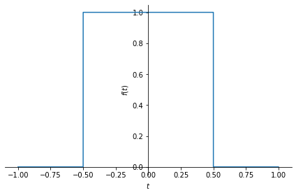
Below we compute the trigonometric Fourier series of the following rectangular pulse signal:

\[\begin{split} x(t) = \begin{cases} 1, & |t| \le 0.5, \\ 0 , & 0.5 \lt |t| \le 1. \\ \end{cases} \end{split}\]

with fundamental period \(2\).

x = sym.Heaviside(t+1/2) - sym.Heaviside(t-1/2)
sym.plot(x, (t, -1, 1))

s = sym.fourier_series(x, (t, -1, 1))

from IPython.display import display
display("a_0:", s.a0)
display("a_n (for n>=1):", s.an)
display("b_n (for n>=1):", s.bn)

_images/ad302fd3b4b38e9c7a245784cc221960357a48cf79166a0e8224c272e41a5e53.png

'a_0:'

\[\displaystyle 0.5\]

'a_n (for n>=1):'

\[\displaystyle \left[\frac{2 \cos{\left(\pi t \right)}}{\pi}, 0, - \frac{2 \cos{\left(3 \pi t \right)}}{3 \pi}, 0, \ldots\right]\]

'b_n (for n>=1):'

\[\displaystyle \left[0, 0, 0, 0, \ldots\right]\]

Exercise: Write a script to convert trigonometric Fourier series coefficients to spectral coefficients (Hint: Section 6.9).