Unit impulse and unit step functions

Unit impulse and unit step functions are two basic building blocks, using which you can create other functions. In the following, we explore these functions and their relations to each other.

Continuous time unit impulse

The continuous time unit impulse is defined as follows:

\[ \delta(t) = \lim_{\Delta \to 0} \delta_{\Delta}(t), \]

where

\[\begin{split} \delta_{\Delta}(t)= \begin{cases} \frac{1}{\Delta} & \text{for $0 < t < \Delta$,}\\ 0 & \text{otherwise.} \end{cases} \end{split}\]

This function is also called the Dirac delta function. Sympy provides an implementation for it, namely DiracDelta:

import sympy as sym
sym.init_printing()

t = sym.symbols('t', real=True)

delta = sym.DiracDelta(t)
delta

We can use this function to check the properties of the unit impulse function.

The area under the unit impulse function is \(1\). The following line of code implements \(\int_{-\infty}^\infty \delta(t) dt\).

sym.integrate(delta, (t, -sym.oo, sym.oo))

When we multiply the unit impulse with a function \(x(t)\) and integrate, we get \(x(0)\):

\[ \int_{-\infty}^{\infty} x(t) \delta(t)dt = x(0). \]

You can check this with

x = sym.Function('x')(t)
sym.integrate(x*delta, (t, -sym.oo, sym.oo))

Another nice property of the unit impulse function is the convolution property:

\[ x(t) = \int_{-\infty}^{\infty} x(\tau) \delta(t-\tau) d\tau. \]

With Sympy, you can take this convolution integral as follows:

tau = sym.symbols('tau', real=True)
sym.integrate(x.subs(t, tau)*delta.subs(t,t-tau), (tau, -sym.oo, sym.oo))

Continuous time unit step

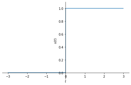
The continuous time unit step function is defined as

\[\begin{split} u(t)=\begin{cases} 1, & \text{for $t \geq 0$,} \\ 0, & \text{otherwise.}\end{cases} \end{split}\]

It is also called the Heaviside step function. Sympy provides this function:

u = sym.Heaviside(t)
u

Sympy uses \(\theta(t)\) to represent the unit step. Let us plot the unit step.

sym.plot(u, (t, -3, 3), ylim=[-0.1, 1.1], ylabel=r'$u(t)$');

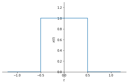
You can easily obtain a rectangular pulse function using two step functions:

rect = sym.Heaviside(t+1/2) - sym.Heaviside(t-1/2)
sym.plot(rect, (t, -1.2, 1.2), ylim=[-0.1, 1.3], ylabel=r'$x(t)$');

Relation between the CT unit impulse and the CT unit step

We can obtain the unit impulse by differentiating the unit step:

\[ \delta(t) = \frac{d u(t)}{dt}. \]

This can be verified using Sympy as follows:

sym.diff(sym.Heaviside(t), t)

In the reverse direction, we can obtain the unit step from the unit impulse by integrating it:

\[ u(t) = \int_{-\infty}^t \delta(\tau) d\tau. \]

To verify this with Sympy, the following line of code should work.

sym.integrate(sym.DiracDelta(t), (t, -sym.oo, t))

Remember, Sympy uses \(\theta(t)\) to represent the unit step, whereas we use the \(u(t)\) notation.

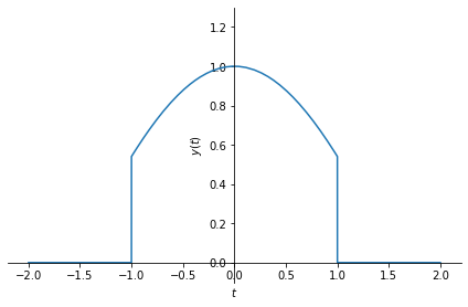
We can use a unit step function or a rectangular pulse to “select” a part of another signal, by multiplying them. An example follows.

# let us mulptiply a cosine signal with a rectangular pulse: 
rect = sym.Heaviside(t+1) - sym.Heaviside(t-1)
y = sym.cos(t)*rect 
sym.plot(y, (t, -2, 2), ylim=[-0.1, 1.3], ylabel=r'$y(t)$');

Discrete time unit impulse

The discrete time unit impulse function is defined as follows:

\[\begin{split} \delta[n]= \begin{cases} 1, & \text{for $n = 0$,}\\ 0, & \text{otherwise.}\end{cases} \end{split}\]

Let us create such a signal and plot it:

import numpy as np
from matplotlib import pyplot as plt 

# define the discrete time unit impulse function
def delta(n): 
    return np.where(n==0.0, 1.0, 0.0) 

# plot the signal in [-3,3]
n = np.arange(-3,4,1)
plt.stem(n, delta(n))
plt.ylabel('$\delta[n]$');

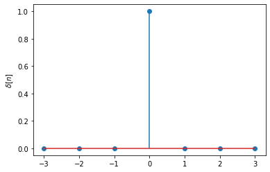
You can plot shifted versions of it:

a = 2 # change this value to see its effect 
plt.stem(n, delta(n-a));

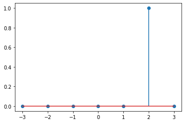
When we multiply a signal with a unit impulse, it “sifts” the corresponding component, that is, \(x[n]\cdot \delta[n-k]\) equals to \(x[k]\) because \(\delta[n-k]\) would be non-zero only at \(n=k\).

Building upon this property, we can express any discrete time signal \(x[n]\) using the convolution sum with \(\delta[n]\) as follows:

\[ x[n]*\delta[n] = x[n] = \sum_{k=-\infty}^{\infty} x[k]\cdot \delta[n-k]. \]

We can test this using numpy’s convolution:

# let's create a discrete time signal by specifying its values for n=0 through
# n=4. For all other values of n, the signal is zero. 
x = [0.1, 0.7, -.2, 0.2, 0.5]

# unit impulse. delta[0] = 1. For all other n, delta is zero
delta = [1]

y = np.convolve(x, delta)
print("x: " , x)
print("convolution result: ", y)

x:  [0.1, 0.7, -0.2, 0.2, 0.5]
convolution result:  [ 0.1  0.7 -0.2  0.2  0.5]

Discrete time unit step

Discrete time unit step function is analytically defined as follows:

\[\begin{split} u[n]=\begin{cases} 1 & \text{for $n \geq 0$}\\ 0, & \text{otherwise.} \end{cases} \end{split}\]

Let us create and plot it.

# define the discrete time unit step function
def u(n): 
    return np.where(n>0.0, 1.0, 0.0) 

# plot the signal in [-5,5]
n = np.arange(-5,6,1)
plt.stem(n, u(n))
plt.ylabel('$u[n]$');

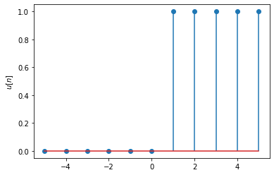
Similar to the continuous time case, we can create a rectangular pulse by subtracting a time-shifted unit step from another time-shifted unit step:

def rect(n): 
    return u(n+2)-u(n-2)

# plot the signal in [-5,5]
n = np.arange(-5,6,1)
plt.stem(n, rect(n))
plt.ylabel('$u[n]$');

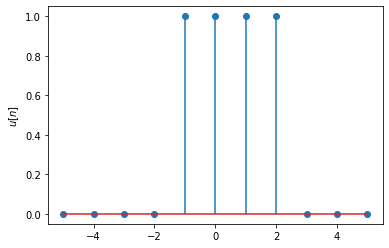
Relation between the DT unit impulse and the DT unit step

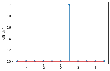
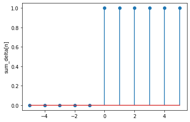
We can obtain the unit step from the unit impulse through summation and the other way around through difference:

\[ u[n]=\sum\limits_{k=0}^{\infty} \delta[n-k] \]

\[ \delta[n] = u[n] - u[n-1] \]

Let us write code to show these two properties.

# define the discrete time unit impulse function
def delta(n): 
    return np.where(n==0.0, 1.0, 0.0) 

# sum the unit impulse
def sum_delta(n): 
    s = 0;
    for k in range(10): # theoretically this summation should go up to 
                        # infinity but we truncate it at some finite value for 
                        # practical purposes. 
        s += delta(n-k)
    return s


# plot the signal in [-5,5]
n = np.arange(-5,6,1)
plt.stem(n, sum_delta(n))
plt.ylabel('sum_delta[n]');

# define the discrete time unit step function
def u(n): 
    return np.where(n>0.0, 1.0, 0.0) 

# the unit step is nothing but: 
def diff_u(n): 
    return u(n)-u(n-1)

# plot the signal in [-5,5]
n = np.arange(-5,6,1)
plt.stem(n, diff_u(n))
plt.ylabel('diff_u[n]');