The complex exponential signal#
As we explained in Chapter 2, the exponential function, \(C e^{\alpha t}\), is one of the most important functions for signals and systems. When the \(\alpha\) is imaginary, we call this function the complex exponential function.
Continuous time complex exponential signal#
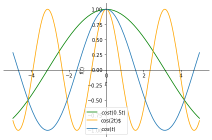
Consider the continuous time exponential signal \(x(t) = e^{j \omega t}\). Using Euler’s formula, we have
\(x(t) = e^{j\omega t} = \cos(\omega t) + j \sin(\omega t)\).
Note that \(x(t)\) is periodic for any value of \(\omega\), as both the real and the imaginary components are periodic. As \(\omega\) is increased, the frequency of \(x(t)\) will increase.
Let us examine its behavior. We will focus only on the real part for ease of visualization but the imaginary part behaves similarly.
import sympy as sym

t = sym.symbols('t', real=True)

# the signal cos(omega t) for different omega values:
x = sym.cos(t)
y = sym.cos(2*t)
z = sym.cos(0.5*t)

# plot
px = sym.plot(x, (t, -5, 5), legend=True, label='$cos(t)$', show=False);
py = sym.plot(y, (t, -5, 5), legend=True, label=r'cos(2t)$', show=False,
              line_color='orange')
pz = sym.plot(z, (t, -5, 5), legend=True, label=r'$cost(0.5t)$', show=False,
              line_color='green')
py.extend(px)
pz.extend(py)
pz.show()
If you run the code below, it will create a slider using which you can change the value of omega using your mouse. It facilitates seeing how the plot changes with different values of omega.
import matplotlib.pyplot as plt
import numpy as np
from ipywidgets import interact

# continuous time signal
def plot_cos(omega):
  t = np.arange(0,4*np.pi, .001)
  x = np.cos(omega*t)
  plt.plot(t,x)
  plt.xlabel('t')
  plt.ylabel('cos($\omega$ t)')
  plt.show()

interact(plot_cos, omega=(0,10,.1));
Discrete time complex exponential signal#
As we mentioned above, the CT exponential signal \(x(t) = e^{j\omega t}\) is periodic for any value of \(\omega\) and as \(\omega\) is increased, the frequency of \(x(t)\) will increase.
However, for the DT signal \(x[n] = e^{j \omega n}\), the situation is different.
Using the Euler’s formula, we can write
\(x[n] = e^{j\omega n} = \cos(\omega n) + j \sin(\omega n).\)
Now let us focus on the real part of \(x[n]\); the imaginary part behaves similarly. Let \(y[n]=\cos(\omega n)\). For \(y[n]\) to be periodic, \(y[n]\) should be equal to \(y[n+N]\) for integer and positive \(N\). For \(y[n+N] = \cos( \omega n + \omega N)\) to be equal to \(y[n]\), we need \(\omega N\) to be an integer multiple of \(2\pi\), since \(\cos\) is periodic with \(2\pi\).
Then, we can write the condition for \(y[n]\) to be periodic as follows:
\(\frac{N}{k} = \frac{2\pi}{\omega}\) where \(N\), \(k\) should be integers, or, equivalently, \(\frac{2\pi}{\omega}\) must be a rational number.
In summary, the frequency of \(x[n]\) will not always increase as \(\omega\) is increased, and for some values of \(\omega\), the signal will not be periodic.
Now let us inspect whether \(y[n]=\cos(\omega n)\) is periodic for two different values of \(\omega = \{1, \frac{\pi}{8}\}\).
import numpy as np
import matplotlib.pyplot as plt

n = np.arange(-20, 20, 1)

# the signal cos(omega n)
omega = 1
x = np.cos(omega*n)

# plot
plt.stem(n,x, linefmt='blue');
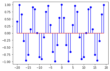
While the plot shows a roughly repeating pattern, it is not possible to draw a certain conclusion from the plot. We should check the condition
\(\frac{N}{k} = \frac{2\pi}{\omega}\).
When \(\omega=1\), \(\frac{N}{k}\) is an irrational number because \(\pi\) is irrational. So, \(y[n]=\cos(n)\) is not a periodic signal.
Let us now inspect \(y[n]\) for \(\omega = \frac{\pi}{8}\).
# the signal cos(omega n)
omega = np.pi/8
x = np.cos(omega*n)

# plot
plt.stem(n,x, linefmt='blue');
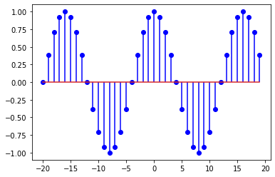
This time the plots looks periodic but again, we should the check periodicity condition:
\(\frac{N}{k} = \frac{2\pi}{\omega} = 16\), which is a rational number, so, \(y[n]=\cos(\frac{\pi}{8}n)\) is periodic.
The following piece of code will let you change omega interactively (through a slider). Observe the behavior of the signal and compare it to that of the CT counterpart above. (Hint: clicking on the slider and then using the arrow keys on your keyboard allows minimal increments for omega.)
# discrete time signal
def plot_cos(omega):
  n = np.arange(-20,20, 1)
  x = np.cos(omega*n)
  plt.stem(n,x);
  plt.xlabel('n')
  plt.ylabel('cos($\omega$ n)')
  plt.show()

interact(plot_cos, omega=(0,100,.01));